The sample size for neuromarketing tests

Anyone who has actually thought about leading or conducting a neuromarketing test or, more a general, a test that involves the collection of psychophysiological data, you will be faced with a fateful question: how many people do I have to recruit for my test why is this sufficiently representative?

To answer this question it is necessary to bother some statistics books, but do not worry… we will not go too far into the dark places of this discipline. We have deliberately simplified the subject to the maximum, so we urge you not to use this content as Bignami for a statistical exam. Rather – as long as you don’t work at ISTAT – take the liberty of making a good impression in front of your colleagues during the break at the coffee machine.

In this article we will limit ourselves to introducing some concepts that will allow you to understand what involves increasing or reducing the number of the sample.

1° Normal distributrion

For those with interviews and questionnaires, know that one could be enough for a neuromarketing test fifteen people probably it will displace it. It will seem strange to you but there is a very simple reason behind it.The object of the investigation is different, just as the type of data that is collected is very different. The psychophysiological data (such as brain waves, pupil size, heart rate, etc.), these are data that are distributed normally. Distributing normally means that if we try to represent them for example, they would look like this graph (Figure 1).

Figure 1. Normal or Gaussian distribution

If this image represented the distribution of the heart rate of the world population we could easily assert that it will be much more likely to find people who have a resting heart rate around 80 beats per minute (middle column broken), compared to those who have 40 of the first columns on the left) or 120 (one of the last columns on the right). The more people there are in that condition, the more that column will be “high”.

2nd The analysis of variance

L‘analysis of variance (ANOVA, ANalysis Of VAriance) is a data analysis technique that allows to verify hypotheses concerning differences between the averages of two or more populations (selected on a sample basis). Always remaining in the heartbeat, if for example we wanted to know how reliable a certain is wrist heart rate monitor in measuring heart rate, it will be sufficient to compare the data recorded simultaneously by the various heart rate monitors and by a medical-derived ECG that will act as a reference measurement.

The greater the difference between the two measurements compared to the reference one, the more unreliable that device will be.

The analysis of variance is a parametric statistical technique which means first of all assume that the variable of interest is normally distributed in the population and that the two samples are randomly extracted from the population. Furthermore the sample size is relevant and in the comparison between several samples the variances must be homogeneous.

Of course, explaining everything there is to know about ANOVA is a lost attempt at the start. This is not the place, but if you want to learn more about it with us, you should know that in TSW we also do training around these issues.

Aware, therefore, that what we have said so far will not be enough to completely clarify your ideas, we present you with an EEG analysis that we conducted on one TV spot lasting 30 seconds.

The analysis of the spots is one of the most interesting services that we can do with the EEG.

In the specific case we have done an ANOVA using the time (30 seconds) as a factor.

Exactly for the more technical: for reasons related to the readability of the chart we have not represented (second by second) the standard errors of the average or the confidence intervals.

The purpose of this article is indeed to make you understand what is the difference in terms of results between a test conducted with 15 and a test with 40 participants. The literature suggests that for similar studies a maximum of 40 participants were employed: therefore we take this numerosity as a reference limit (Ohme et al., 2009; 2010).

In particular we will magnify the variations in the levels of engagement, deriving from the brainwave analysis (McMahan et al., 2015) and the considerations that follow, gradually increasing the sample size (from 15 to 40 participants).

Below is the graphic representation of the average level of engagement derived from the EEG analysis made on the same TV spot for 15, 20, 30 and 40 participants.

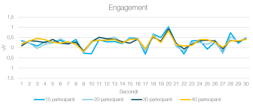
Figure 2. Average trend of the Engagement level for analysis groups composed of 15, 20, 30 and 40 participants respectively

3rd The Correlation

The correlation expresses the relationship existing between two variables. This value varies between –1.00 (negative correlation) and +1.00 (positive correlation). A correlation equal to 0 indicates that there is no relationship between the two variables. Simplifying as much as possible, a correlation can be considered positive and strong if it reaches values ​​above 0.70.

The table below explains exactly what happens from a correlation point of view with samples ranging from 5 to 40 people.

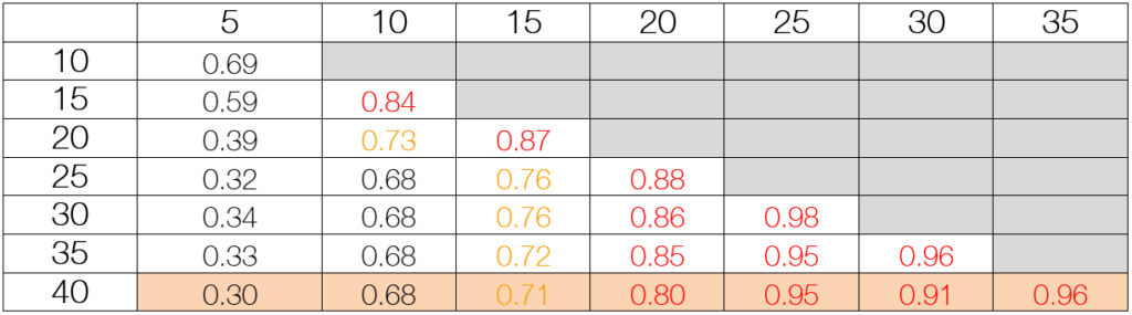
Table 1.

Correlation matrix

Let’s look at how the groups behave with respect to the analysis made with 40 participants (Table 1). As you can see the analysis with 5 or 10 participants is not sufficiently correlated with the analysis carried out with 40. But already with 15 participants we know we are on the right path. With 20 participants we achieve excellent values ​​that allow us to say that increasing the number of users (up to 40) does not provide real benefits that justify the investment.

As shown in Figure 2, the performances and trends are quite similar between them. However, graphic perception does not always go hand in hand with statistics. So we went to evaluate second by second which moments differed from the average level of engagement of the whole experience, or what we call peaks.

There table below it simplifies the meticulous analysis work and allows a comparison of the results that could be obtained with the different numbers easily.

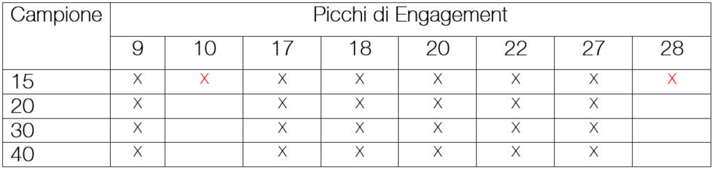
Table 2. Peaks of engagement for different champions. In the column the seconds in which engagement peaks were observed, in line the number of participants.

As you can see, for this spot, the analysis carried out with a sample of 20 people allows us to identify the same problems that derive from the analysis made with twice as many users (40).

It is interesting to note how with 15 participants highlight all the critical issues, overestimating the differences for the peaks recorded at the second 10 and the second 28 (no longer observable from the analyzes made with 20 participants). If on the one hand it is true that already with 15 we have strongly correlated results (i.e. 0.71) with a sample of 40, on the other this does not mean that there are no differences between the two observations.

In conclusion, we hope to have made you understand (without too many headaches) that the choice of numerosity does not depend on personal considerations but on statistical considerations closely linked to the aims and object of the investigation. Finally it seems important to underline that these considerations can be extended to all the groups that we wish to analyze. For example if we wanted to know if there are differences between males and females, we will need at least 15/20 male and as many female people. Each further comparison will respect the same rules. At this point we should have understood that the choice of the number of a sample depends above all on the objectives what we ask ourselves: the more we want to know, the bigger the sample will have to be recruited. But we can finally forget about the numbers needed for interviews!

Bibliography

McMahan, T., Parberry, I., & Parsons, T. D. (2015, June). Evaluating Electroencephalography Engagement Indices During Video Game Play. In FDG.

Ohme, R., Reykowska, D., Wiener, D., & Choromanska, A. (2009). Analysis of neurophysiological reactions to advertising stimuli by means of EEG and galvanic skin response measures. Journal of Neuroscience, Psychology, and Economics, 2(1), 21.

Ohme, R., Reykowska, D., Wiener, D., & Choromanska, A. (2010). Application of frontal EEG asymmetry to advertising research. Journal of Economic Psychology, 31(5), 785-793.